paper

Introduction

Contrastive Learning 受益于区分hard negatives (最相似的negative pairs)， 但是其他领域的hard negative mining方法不适用于graph。 对于GCL来说大量embedding之后的hard negatives实际上是false negatives。如左图所示，对于CV上的SimCLR，它所学到的高相似度的negatives中，True negatives 和False negatives数量相当，那么从高相似度的negatives中采样到true negatives的概率更大。然而对于GCL方法GCA来说，是每个anchor节点将其他所有（inter/intra）节点作为negatives，使得在训练过程中与它同类的节点也变成anchor的negatives，这些negatives是false negatives。对于GCA，高相似度的negatives中false negatives的数量远多于true negatives，所以直接采样高相似度的negatives作为hard negatives来针对性的判别他们，会导致同类节点的embedding相互远离。这是传统的hard negatives mining方法在graph domain失效的原因。

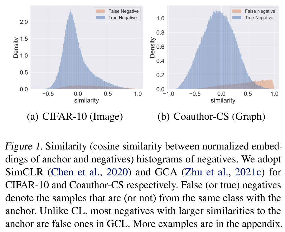
为了解决这个问题， 本文提出利用Beta mixture model来估计对于一个anchor node，它的一个negatve是true negative的概率，结合相似度，来衡量该negative的hardness。即与anchor node相似度越高，且它是true negative的概率越大，那么该节点的hardness越高。

Methodology

GCL

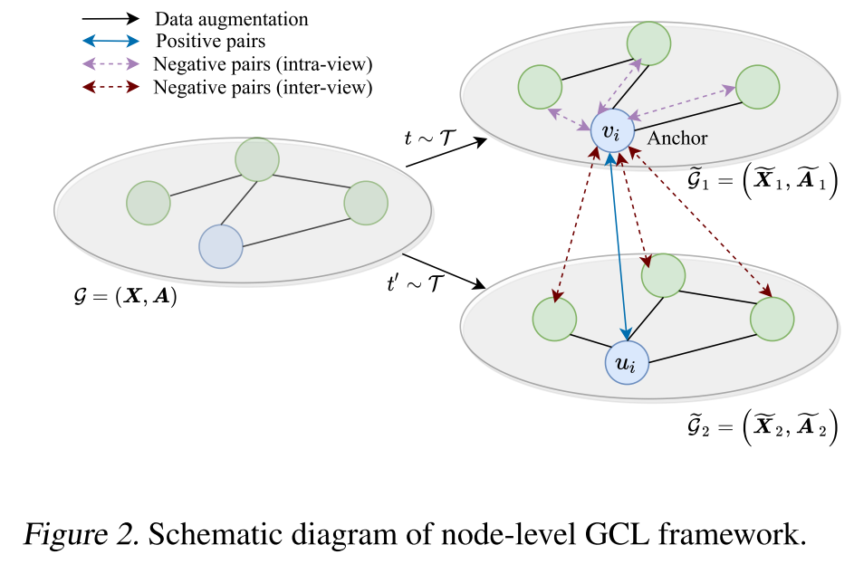
如上图所示，InfoNCE将跨图same node视为positives，其他节点对视为negatives，GCL的目标函数如下： $$ \begin{aligned} \ell\left(\boldsymbol{u}_{i},\boldsymbol{v}_{i}\right)= \log \frac{e^{\theta\left(\boldsymbol{u}_{i}, \boldsymbol{v}_{i}\right) / \tau}}{\underbrace{e^{\theta\left(\boldsymbol{u}_{i}, \boldsymbol{v}_{i}\right) / \tau}}_{\text{positive pair }}+\underbrace{\sum_{k\neq i}e^{\theta\left(\boldsymbol{u}_{i}, \boldsymbol{v}_{k}\right) / \tau}}_{\text{inter-view negative pairs}}+\underbrace{\sum_{k\neq i}e^{\theta\left(\boldsymbol{u}_{i}, \boldsymbol{u}_{k}\right) / \tau}}_{\text{intra-view negative pairs}}}, \end{aligned} $$ Overall objective定义在所有跨图same node pairs上： $$ \mathcal{J}=-\frac{1}{2 N} \sum_{i=1}^N\left[\ell\left(\boldsymbol{u}_{\boldsymbol{i}}, \boldsymbol{v}_{\boldsymbol{i}}\right)+\ell\left(\boldsymbol{v}_{\boldsymbol{i}}, \boldsymbol{u}_{\boldsymbol{i}}\right)\right] $$ 如果将GCA中的2层shared GNN替换为MLP，那么contrastive learning将不存在Message Passing，这样得到的true/false negative分布如(b)所示，可以看出Message Passing是GCL和CL之间产生区别关键因素。直观上，MP将anchor与相邻的negatives拉近，而相邻的negatives大多为False negatives（Homophily），所以GCL得到的高相似度negatives中false negatives要远多于True negatives。

Theorem 3.1: $\mathcal{G}$ is a non-bipartile and connected graph with $N$ nodes $\mathcal{V}=\left\{v_1, \ldots, v_N\right\}$ and $\boldsymbol{X}_i^{(\tau)}$ is the embedding of node $v_i$ after $\tau$ tims message passing. For large enough $\tau$, $$ \left|\left|\boldsymbol{X}_i^{(\tau)}-\boldsymbol{X}_j^{(\tau)}\right|\right|_2 \leq\left|\left|\boldsymbol{X}_i^{(0)}-\boldsymbol{X}_j^{(0)}\right|\right|_2 $$ 该定理说明了Message passing之后，不同节点间的距离会变小。

ProGCL

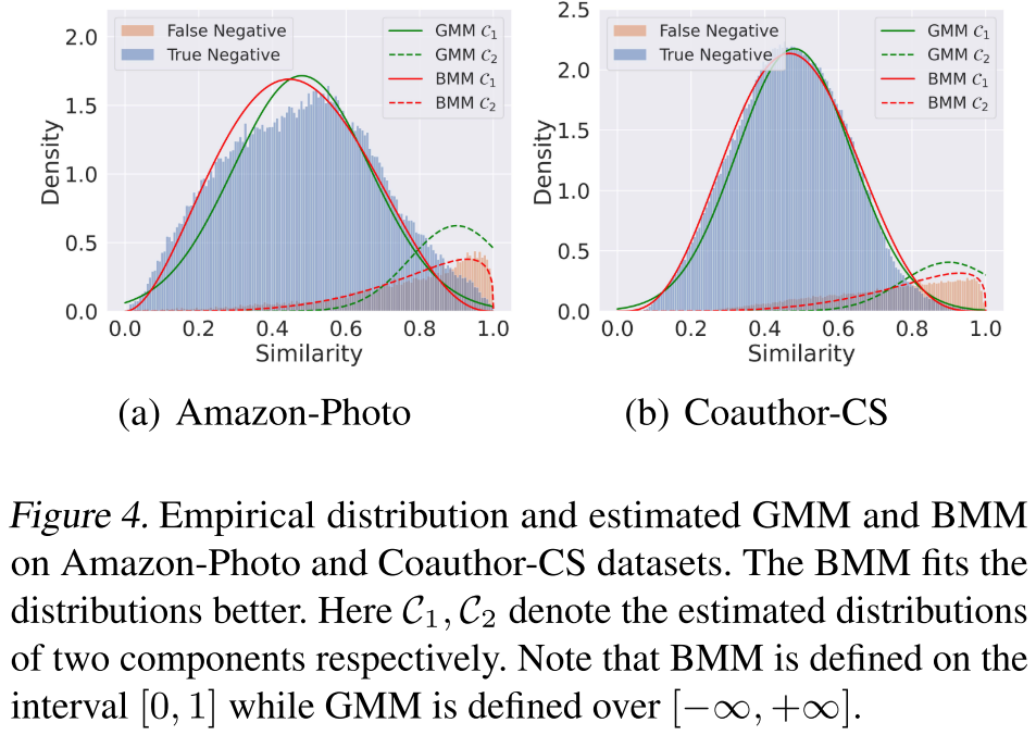
Figure 4描述了negatives相似度的直方图分布，即每个相似度下true/false negatives的相对数量。例如Figure 4（a），对于true negatives，高相似度的true negatives较少，中等相似度的true negatives较多；对于False negatives，大多相似度较高。所以直接采样高相似度的negatives作为hard negatives很容易采样到false negatives。那么随机采样一个相似度$s$的概率有该相似度在true negatives中的采样概率和在false negatives采样概率共同决定。因此相似度分布可以建模为mixture model。本文用Beta distribution来建模true/false negatives的相似度分布。beta distribution的pdf为： $$ p(s \mid \alpha, \beta)=\frac{\Gamma(\alpha+\beta)}{\Gamma(\alpha) \Gamma(\beta)} s^{\alpha-1}(1-s)^{\beta-1}, $$ 其中$\alpha, \beta >0$ 是beta distribution的参数，$\Gamma(\cdot)$ 是gamma function。对于$C$个beta distribution的mixture model，相似度$s$在该mixture model中的概率为$s$在true negatives 相似度分布中的概率和false negatives相似度分布中的概率的加权： $$ p(s)=\sum_{c=1}^{C} \lambda_{c} p(s \mid \alpha_c, \beta_c), $$ 其中$\lambda_c$是mixture coefficients。下面要做的就是通过EM算法来优化两beta mixture model的参数，包括两个beta distribution的$\alpha, \beta$参数以及mixture coefficient，使得GCL学习得到的negatives similarities从改mixture model中采样的概率最大，即优化mixture model这个混合概率分布，使其符合所有negatives similarity分布。例如总共有10000个negatives（true+false），这一万个similarity分布要符合分布$p(s)$。用EM算法来优化mixture model $p(s)$时，E-step要计算后验： $$ p(c\mid s)=\frac{\lambda_{c} p\left(s \mid \alpha_{c}, \beta_{c}\right)}{\sum_{j=1}^{C} \lambda_{j} p\left(s \mid \alpha_{j}, \beta_{j}\right)}. $$ 其中$c$为latent variable。然而优化Beta Mixture Model使其你和所有negatives的similarity分布是计算量巨大的，为了解决这个问题每次迭代只采样$M$ ($M \ll N^2$)个相似度来的分布来优化BMM，使其你和这$M$个相似度的分布。首先计算$M$个相似度在每个beta distribution上的weighted average $\bar{s}_c$以及variance $v_c^2$： $$ \bar{s}_c=\frac{\sum_{i=1}^M p\left(c \mid s_i\right) s_i}{\sum_{i=1}^M p\left(c \mid s_i\right)}, \quad v_c^2=\frac{\sum_{i=1}^M p\left(c \mid s_i\right)\left(s_i-\bar{s}_c\right)^2}{\sum_{i=1}^M p\left(c \mid s_i\right)} . $$ 在M-step，如下优化BMM的参数 $\alpha_c, \beta_c, \lambda_c$使得BMM符合$M$个similarity的分布： $$ \alpha_c=\bar{s}_c\left(\frac{\bar{s}_c\left(1-\bar{s}_c\right)}{v_c^2}-1\right), \quad \beta_c=\frac{\alpha_c\left(1-\bar{s}_c\right)}{\bar{s}_c}，\quad \lambda_c=\frac{1}{M} \sum_{i=1}^M p\left(c \mid s_i\right) $$ 这样通过E-step计算后验和average, variance，M-step基于average,variance和后验更新BMM的参数，循环迭代$I=10$次后，可以得到拟合输入negatives similarity的BMM分布的参数。最终，得到关于相似度$s$的BMM$p(s)$后，构成$p(s)$的两个分布即给定negative similarity $s$，该negative是true negative/false negative的概率为： $$ p(c \mid s)=\frac{\lambda_c p\left(s \mid \alpha_c, \beta_c\right)}{p(s)} $$

ProGCL-weight

对于一对negative pair，$\boldsymbol{u}_i$为anchor和他的inter-view $\boldsymbol{v}_k$，他们的相似度$s_{ik}$在true negative分布中的概率为$p(c_t|s_{ik})$，概率越大越可能是true negative，同时$s_{ik}$越大越hardness。所以在Contrastive loss中，越hard的true negative要被赋予越大的权重，使得被判别区分。negative pair权重为： $$ w(i, k)=\frac{p\left(c_t \mid s_{i k}\right) s_{i k}}{\frac{1}{N-1} \sum_{j \neq i}\left[p\left(c_t \mid s_{i j}\right) s_{i j}\right]} $$ 在Contrastive objective中对negatives加权： $$ \ell_w\left(\boldsymbol{u}_{i}, \boldsymbol{v}_{i}\right)= \log \frac{e^{\frac{\theta\left(\boldsymbol{u}_{i}, \boldsymbol{v}_{i}\right)}{ \tau}}}{\underbrace{e^{\frac{\theta\left(\boldsymbol{u}_{i}, \boldsymbol{v}_{i}\right)}{\tau}}}_{\text{positive pair }}+\underbrace{\sum_{k\neq i}w(i,k)e^{\frac{\theta\left(\boldsymbol{u}_{i}, \boldsymbol{v}_{k}\right)}{\tau}}}_{\text{inter-view negative pairs}}+\underbrace{\sum_{k\neq i}w(i,k)e^{\frac{\theta\left(\boldsymbol{u}_{i}, \boldsymbol{u}_{k}\right)} {\tau}}}_{\text{intra-view negative pairs}}}, $$